Modeling ART interruptions

New in v1.5.3

This example shows how to model exogenous shocks to ART coverage — for instance, supply chain disruptions, conflict, or policy changes that temporarily reduce ART availability.

We’ll:

Set up a baseline HIV sim with historical ART coverage data
Build scenario-specific coverage DataFrames that introduce interruptions
Run and compare counterfactual scenarios

Key concepts: mixed-format coverage (n/p), coverage DataFrames, scenario comparison.

Setup

We’ll use a simplified model with 2,000 agents running from 2000 to 2035. In a real analysis you’d use more agents and location-specific demographic data.

import numpy as np
import pandas as pd
import sciris as sc
import starsim as ss
import stisim as sti
import hivsim
import matplotlib.pyplot as plt

Building baseline coverage

First, let’s create a realistic ART scale-up trajectory. In practice you’d load this from a CSV, but we’ll build it programmatically here.

# Historical ART numbers (absolute counts) representing scale-up in a
# population of ~2,000 with ~15% HIV prevalence (~300 PLHIV).
# By 2023, ~650 on ART (accounting for population growth over 23 years).
years_hist = np.arange(2000, 2023)
n_art_hist = [0, 1, 4, 10, 20, 40, 70, 110, 155, 210, 265, 315,
              365, 405, 440, 475, 510, 540, 565, 590, 610, 630, 650]

# Build a dual-column DataFrame: n_art for historical, p_art for projected
baseline_df = pd.DataFrame(index=years_hist)
baseline_df['n_art'] = n_art_hist

# From 2023 onward, switch to proportion-based targets
for year in range(2023, 2036):
    baseline_df.loc[year, 'p_art'] = 0.90

print(baseline_df.tail(10))

      n_art  p_art
2026    NaN    0.9
2027    NaN    0.9
2028    NaN    0.9
2029    NaN    0.9
2030    NaN    0.9
2031    NaN    0.9
2032    NaN    0.9
2033    NaN    0.9
2034    NaN    0.9
2035    NaN    0.9

When you pass a DataFrame with both n_art and p_art columns, STIsim automatically uses n_art where available and falls back to p_art for years where n_art is NaN. This is controlled by the format_priority parameter (default: 'n').

Defining interruption scenarios

Now let’s define a helper that modifies the coverage DataFrame to simulate a temporary ART interruption — a period where ART coverage drops by some fraction.

def make_interruption(base_df, shock_year, reduction, duration):
    """
    Create a coverage DataFrame with an ART interruption.
    
    Args:
        base_df:     baseline coverage DataFrame
        shock_year:  year the interruption begins
        reduction:   fractional reduction (e.g. 0.3 = 30% drop)
        duration:    number of years the interruption lasts
    
    Returns:
        Modified DataFrame with reduced coverage during the shock period.
    """
    df = base_df.copy()
    for year in range(shock_year, shock_year + duration):
        if year in df.index:
            # Reduce whichever column is active
            if pd.notna(df.loc[year, 'n_art']):
                df.loc[year, 'n_art'] *= (1 - reduction)
            elif pd.notna(df.loc[year, 'p_art']):
                df.loc[year, 'p_art'] *= (1 - reduction)
    return df

# Define scenarios: baseline + three interruption severities
scenarios = {
    'Baseline':          baseline_df,
    '20% drop, 2 years': make_interruption(baseline_df, 2025, 0.2, 2),
    '50% drop, 2 years': make_interruption(baseline_df, 2025, 0.5, 2),
    '50% drop, 5 years': make_interruption(baseline_df, 2025, 0.5, 5),
}

Running the scenarios

We run each scenario using hivsim.demo with the same random seed so differences are due to the intervention, not stochastic variation.

results = {}
seed = 42

for label, cov_df in scenarios.items():
    sim = hivsim.demo('simple', run=False, plot=False, n_agents=2_000, stop=2035,
                       verbose=-1, rand_seed=seed)
    
    # Replace the default ART with our scenario-specific coverage
    sim.pars.interventions = [
        sti.HIVTest(name='hiv_test', test_prob_data=0.3),
        sti.ART(coverage=cov_df),
    ]
    sim.run()
    results[label] = sim
    print(f'{label}: {sim.results.hiv.n_on_art[-1]:.0f} on ART at end')

Initializing sim with 2000 agents

  Running 2000.01.01 ( 0/421) (0.00 s)  ———————————————————— 0%

  Running 2001.01.01 (12/421) (0.54 s)  ———————————————————— 3%

  Running 2002.01.01 (24/421) (0.73 s)  •——————————————————— 6%

  Running 2003.01.01 (36/421) (0.93 s)  •——————————————————— 9%

  Running 2004.01.01 (48/421) (1.12 s)  ••—————————————————— 12%

  Running 2005.01.01 (60/421) (1.32 s)  ••—————————————————— 14%

  Running 2006.01.01 (72/421) (1.51 s)  •••————————————————— 17%

  Running 2007.01.01 (84/421) (1.71 s)  ••••———————————————— 20%

  Running 2008.01.01 (96/421) (1.90 s)  ••••———————————————— 23%

  Running 2009.01.01 (108/421) (2.10 s)  •••••——————————————— 26%

  Running 2010.01.01 (120/421) (2.29 s)  •••••——————————————— 29%

  Running 2011.01.01 (132/421) (2.49 s)  ••••••—————————————— 32%

  Running 2012.01.01 (144/421) (2.68 s)  ••••••—————————————— 34%

  Running 2013.01.01 (156/421) (2.87 s)  •••••••————————————— 37%

  Running 2014.01.01 (168/421) (3.07 s)  ••••••••———————————— 40%

  Running 2015.01.01 (180/421) (3.26 s)  ••••••••———————————— 43%

  Running 2016.01.01 (192/421) (3.46 s)  •••••••••——————————— 46%

  Running 2017.01.01 (204/421) (3.65 s)  •••••••••——————————— 49%

  Running 2018.01.01 (216/421) (3.85 s)  ••••••••••—————————— 52%

  Running 2019.01.01 (228/421) (4.05 s)  ••••••••••—————————— 54%

  Running 2020.01.01 (240/421) (4.25 s)  •••••••••••————————— 57%

  Running 2021.01.01 (252/421) (4.45 s)  ••••••••••••———————— 60%

  Running 2022.01.01 (264/421) (4.65 s)  ••••••••••••———————— 63%

  Running 2023.01.01 (276/421) (4.85 s)  •••••••••••••——————— 66%

  Running 2024.01.01 (288/421) (5.05 s)  •••••••••••••——————— 69%

  Running 2025.01.01 (300/421) (5.26 s)  ••••••••••••••—————— 71%

  Running 2026.01.01 (312/421) (5.46 s)  ••••••••••••••—————— 74%

  Running 2027.01.01 (324/421) (5.67 s)  •••••••••••••••————— 77%

  Running 2028.01.01 (336/421) (5.87 s)  ••••••••••••••••———— 80%

  Running 2029.01.01 (348/421) (6.08 s)  ••••••••••••••••———— 83%

  Running 2030.01.01 (360/421) (6.28 s)  •••••••••••••••••——— 86%

  Running 2031.01.01 (372/421) (6.49 s)  •••••••••••••••••——— 89%

  Running 2032.01.01 (384/421) (6.69 s)  ••••••••••••••••••—— 91%

  Running 2033.01.01 (396/421) (6.90 s)  ••••••••••••••••••—— 94%

  Running 2034.01.01 (408/421) (7.11 s)  •••••••••••••••••••— 97%

  Running 2035.01.01 (420/421) (7.32 s)  •••••••••••••••••••• 100%

Baseline: 45 on ART at end
Initializing sim with 2000 agents

  Running 2000.01.01 ( 0/421) (0.00 s)  ———————————————————— 0%

  Running 2001.01.01 (12/421) (0.19 s)  ———————————————————— 3%

  Running 2002.01.01 (24/421) (0.38 s)  •——————————————————— 6%

  Running 2003.01.01 (36/421) (0.58 s)  •——————————————————— 9%

  Running 2004.01.01 (48/421) (0.78 s)  ••—————————————————— 12%

  Running 2005.01.01 (60/421) (0.97 s)  ••—————————————————— 14%

  Running 2006.01.01 (72/421) (1.16 s)  •••————————————————— 17%

  Running 2007.01.01 (84/421) (1.36 s)  ••••———————————————— 20%

  Running 2008.01.01 (96/421) (1.55 s)  ••••———————————————— 23%

  Running 2009.01.01 (108/421) (1.75 s)  •••••——————————————— 26%

  Running 2010.01.01 (120/421) (1.95 s)  •••••——————————————— 29%

  Running 2011.01.01 (132/421) (2.14 s)  ••••••—————————————— 32%

  Running 2012.01.01 (144/421) (2.34 s)  ••••••—————————————— 34%

  Running 2013.01.01 (156/421) (2.53 s)  •••••••————————————— 37%

  Running 2014.01.01 (168/421) (2.72 s)  ••••••••———————————— 40%

  Running 2015.01.01 (180/421) (2.91 s)  ••••••••———————————— 43%

  Running 2016.01.01 (192/421) (3.11 s)  •••••••••——————————— 46%

  Running 2017.01.01 (204/421) (3.30 s)  •••••••••——————————— 49%

  Running 2018.01.01 (216/421) (3.50 s)  ••••••••••—————————— 52%

  Running 2019.01.01 (228/421) (3.70 s)  ••••••••••—————————— 54%

  Running 2020.01.01 (240/421) (3.90 s)  •••••••••••————————— 57%

  Running 2021.01.01 (252/421) (4.10 s)  ••••••••••••———————— 60%

  Running 2022.01.01 (264/421) (4.31 s)  ••••••••••••———————— 63%

  Running 2023.01.01 (276/421) (4.50 s)  •••••••••••••——————— 66%

  Running 2024.01.01 (288/421) (4.71 s)  •••••••••••••——————— 69%

  Running 2025.01.01 (300/421) (4.91 s)  ••••••••••••••—————— 71%

  Running 2026.01.01 (312/421) (5.12 s)  ••••••••••••••—————— 74%

  Running 2027.01.01 (324/421) (5.32 s)  •••••••••••••••————— 77%

  Running 2028.01.01 (336/421) (5.52 s)  ••••••••••••••••———— 80%

  Running 2029.01.01 (348/421) (5.73 s)  ••••••••••••••••———— 83%

  Running 2030.01.01 (360/421) (5.94 s)  •••••••••••••••••——— 86%

  Running 2031.01.01 (372/421) (6.14 s)  •••••••••••••••••——— 89%

  Running 2032.01.01 (384/421) (6.35 s)  ••••••••••••••••••—— 91%

  Running 2033.01.01 (396/421) (6.56 s)  ••••••••••••••••••—— 94%

  Running 2034.01.01 (408/421) (6.77 s)  •••••••••••••••••••— 97%

  Running 2035.01.01 (420/421) (6.98 s)  •••••••••••••••••••• 100%

20% drop, 2 years: 45 on ART at end
Initializing sim with 2000 agents

  Running 2000.01.01 ( 0/421) (0.00 s)  ———————————————————— 0%

  Running 2001.01.01 (12/421) (0.19 s)  ———————————————————— 3%

  Running 2002.01.01 (24/421) (0.38 s)  •——————————————————— 6%

  Running 2003.01.01 (36/421) (0.58 s)  •——————————————————— 9%

  Running 2004.01.01 (48/421) (0.78 s)  ••—————————————————— 12%

  Running 2005.01.01 (60/421) (0.97 s)  ••—————————————————— 14%

  Running 2006.01.01 (72/421) (1.16 s)  •••————————————————— 17%

  Running 2007.01.01 (84/421) (1.36 s)  ••••———————————————— 20%

  Running 2008.01.01 (96/421) (1.55 s)  ••••———————————————— 23%

  Running 2009.01.01 (108/421) (1.75 s)  •••••——————————————— 26%

  Running 2010.01.01 (120/421) (1.94 s)  •••••——————————————— 29%

  Running 2011.01.01 (132/421) (2.14 s)  ••••••—————————————— 32%

  Running 2012.01.01 (144/421) (2.33 s)  ••••••—————————————— 34%

  Running 2013.01.01 (156/421) (2.53 s)  •••••••————————————— 37%

  Running 2014.01.01 (168/421) (2.72 s)  ••••••••———————————— 40%

  Running 2015.01.01 (180/421) (2.91 s)  ••••••••———————————— 43%

  Running 2016.01.01 (192/421) (3.11 s)  •••••••••——————————— 46%

  Running 2017.01.01 (204/421) (3.30 s)  •••••••••——————————— 49%

  Running 2018.01.01 (216/421) (3.50 s)  ••••••••••—————————— 52%

  Running 2019.01.01 (228/421) (3.70 s)  ••••••••••—————————— 54%

  Running 2020.01.01 (240/421) (3.90 s)  •••••••••••————————— 57%

  Running 2021.01.01 (252/421) (4.10 s)  ••••••••••••———————— 60%

  Running 2022.01.01 (264/421) (4.30 s)  ••••••••••••———————— 63%

  Running 2023.01.01 (276/421) (4.50 s)  •••••••••••••——————— 66%

  Running 2024.01.01 (288/421) (4.71 s)  •••••••••••••——————— 69%

  Running 2025.01.01 (300/421) (4.91 s)  ••••••••••••••—————— 71%

  Running 2026.01.01 (312/421) (5.12 s)  ••••••••••••••—————— 74%

  Running 2027.01.01 (324/421) (5.32 s)  •••••••••••••••————— 77%

  Running 2028.01.01 (336/421) (5.53 s)  ••••••••••••••••———— 80%

  Running 2029.01.01 (348/421) (5.73 s)  ••••••••••••••••———— 83%

  Running 2030.01.01 (360/421) (5.94 s)  •••••••••••••••••——— 86%

  Running 2031.01.01 (372/421) (6.15 s)  •••••••••••••••••——— 89%

  Running 2032.01.01 (384/421) (6.36 s)  ••••••••••••••••••—— 91%

  Running 2033.01.01 (396/421) (6.56 s)  ••••••••••••••••••—— 94%

  Running 2034.01.01 (408/421) (6.77 s)  •••••••••••••••••••— 97%

  Running 2035.01.01 (420/421) (6.98 s)  •••••••••••••••••••• 100%

50% drop, 2 years: 46 on ART at end
Initializing sim with 2000 agents

  Running 2000.01.01 ( 0/421) (0.00 s)  ———————————————————— 0%

  Running 2001.01.01 (12/421) (0.19 s)  ———————————————————— 3%

  Running 2002.01.01 (24/421) (0.38 s)  •——————————————————— 6%

  Running 2003.01.01 (36/421) (0.58 s)  •——————————————————— 9%

  Running 2004.01.01 (48/421) (0.77 s)  ••—————————————————— 12%

  Running 2005.01.01 (60/421) (0.96 s)  ••—————————————————— 14%

  Running 2006.01.01 (72/421) (1.16 s)  •••————————————————— 17%

  Running 2007.01.01 (84/421) (1.35 s)  ••••———————————————— 20%

  Running 2008.01.01 (96/421) (1.55 s)  ••••———————————————— 23%

  Running 2009.01.01 (108/421) (1.75 s)  •••••——————————————— 26%

  Running 2010.01.01 (120/421) (1.94 s)  •••••——————————————— 29%

  Running 2011.01.01 (132/421) (2.14 s)  ••••••—————————————— 32%

  Running 2012.01.01 (144/421) (2.33 s)  ••••••—————————————— 34%

  Running 2013.01.01 (156/421) (2.52 s)  •••••••————————————— 37%

  Running 2014.01.01 (168/421) (2.72 s)  ••••••••———————————— 40%

  Running 2015.01.01 (180/421) (2.91 s)  ••••••••———————————— 43%

  Running 2016.01.01 (192/421) (3.10 s)  •••••••••——————————— 46%

  Running 2017.01.01 (204/421) (3.29 s)  •••••••••——————————— 49%

  Running 2018.01.01 (216/421) (3.49 s)  ••••••••••—————————— 52%

  Running 2019.01.01 (228/421) (3.69 s)  ••••••••••—————————— 54%

  Running 2020.01.01 (240/421) (3.89 s)  •••••••••••————————— 57%

  Running 2021.01.01 (252/421) (4.09 s)  ••••••••••••———————— 60%

  Running 2022.01.01 (264/421) (4.29 s)  ••••••••••••———————— 63%

  Running 2023.01.01 (276/421) (4.49 s)  •••••••••••••——————— 66%

  Running 2024.01.01 (288/421) (4.70 s)  •••••••••••••——————— 69%

  Running 2025.01.01 (300/421) (4.90 s)  ••••••••••••••—————— 71%

  Running 2026.01.01 (312/421) (5.11 s)  ••••••••••••••—————— 74%

  Running 2027.01.01 (324/421) (5.31 s)  •••••••••••••••————— 77%

  Running 2028.01.01 (336/421) (5.51 s)  ••••••••••••••••———— 80%

  Running 2029.01.01 (348/421) (5.72 s)  ••••••••••••••••———— 83%

  Running 2030.01.01 (360/421) (5.92 s)  •••••••••••••••••——— 86%

  Running 2031.01.01 (372/421) (6.13 s)  •••••••••••••••••——— 89%

  Running 2032.01.01 (384/421) (6.34 s)  ••••••••••••••••••—— 91%

  Running 2033.01.01 (396/421) (6.54 s)  ••••••••••••••••••—— 94%

  Running 2034.01.01 (408/421) (6.76 s)  •••••••••••••••••••— 97%

  Running 2035.01.01 (420/421) (6.97 s)  •••••••••••••••••••• 100%

50% drop, 5 years: 46 on ART at end

Comparing outcomes

Let’s visualize the impact of ART interruptions on treatment numbers and new infections.

colors = sc.gridcolors(4)

with sc.options.with_style('fancy'):
    fig, axes = plt.subplots(1, 2, figsize=(12, 5))

    # Left panel: ART coverage over time
    for (label, sim), color in zip(results.items(), colors):
        axes[0].plot(sim.t.yearvec, sim.results.hiv.n_on_art, label=label, color=color, lw=2)
    axes[0].axvspan(2025, 2030, alpha=0.1, color='red', zorder=0)
    axes[0].set_xlabel('Year')
    axes[0].set_ylabel('People on ART')
    axes[0].set_title('ART coverage')
    axes[0].legend(fontsize=9)

    # Right panel: total new infections during 2025–2030
    labels, totals, bar_colors = [], [], []
    for (label, sim), color in zip(results.items(), colors):
        mask = (sim.t.yearvec >= 2025) & (sim.t.yearvec < 2030)
        totals.append(float(sim.results.hiv.new_infections[mask].sum()))
        labels.append(label)
        bar_colors.append(color)
    axes[1].bar(labels, totals, color=bar_colors, edgecolor='white', linewidth=0.5)
    axes[1].set_ylabel('Total new HIV infections')
    axes[1].set_title('New infections during 2025–2030')
    axes[1].tick_params(axis='x', rotation=20)

    sc.figlayout()
    plt.show()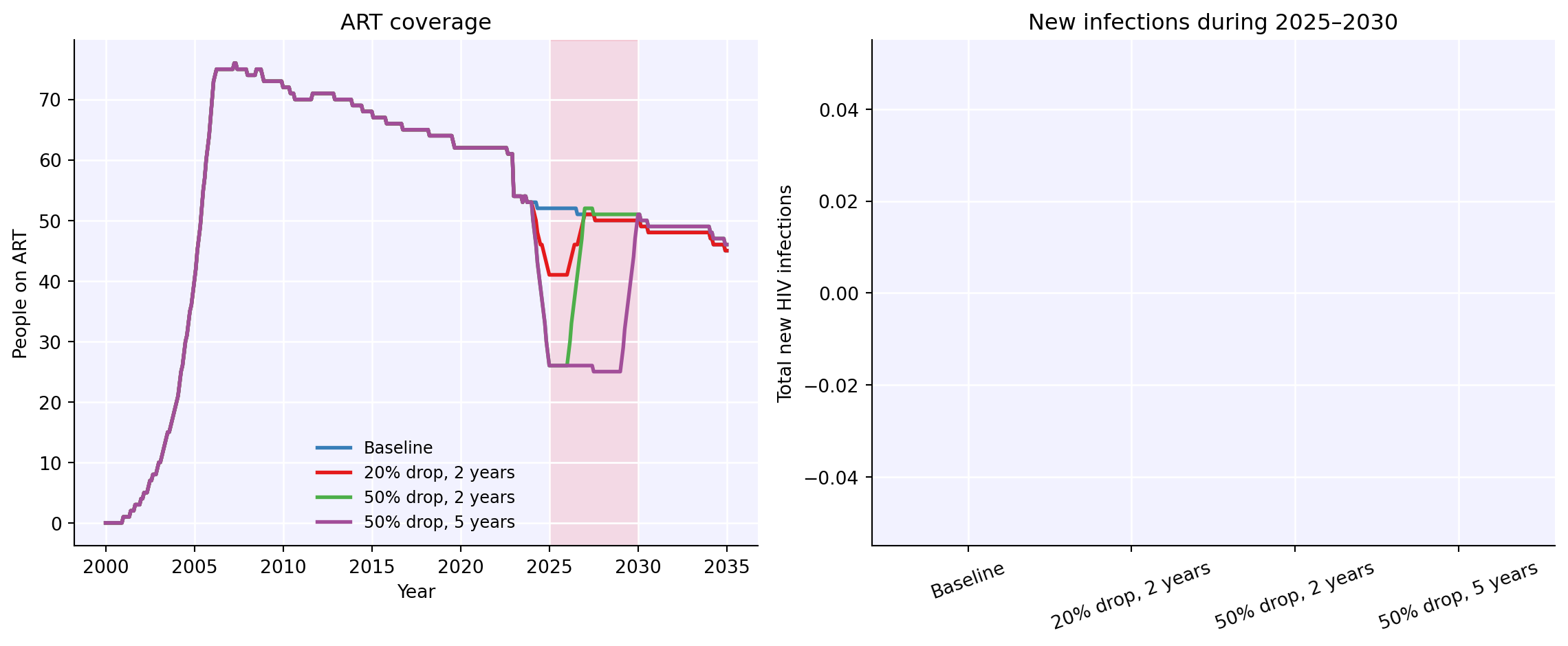

Key takeaways

Mixed-format coverage lets you combine historical data (absolute numbers) with projected targets (proportions) in a single DataFrame
Scenario analysis is straightforward: modify the coverage DataFrame and re-run
The format_priority parameter controls which column takes precedence when both n_art and p_art are present for the same year
For smoother transitions between data points, use the smoothness parameter: sti.ART(coverage=df, smoothness=5)