This tutorial shows how to add testing and treatment interventions to an STIsim simulation. We’ll start with a simple gonorrhea example, then show how HIV interventions work.
Simple STI treatment
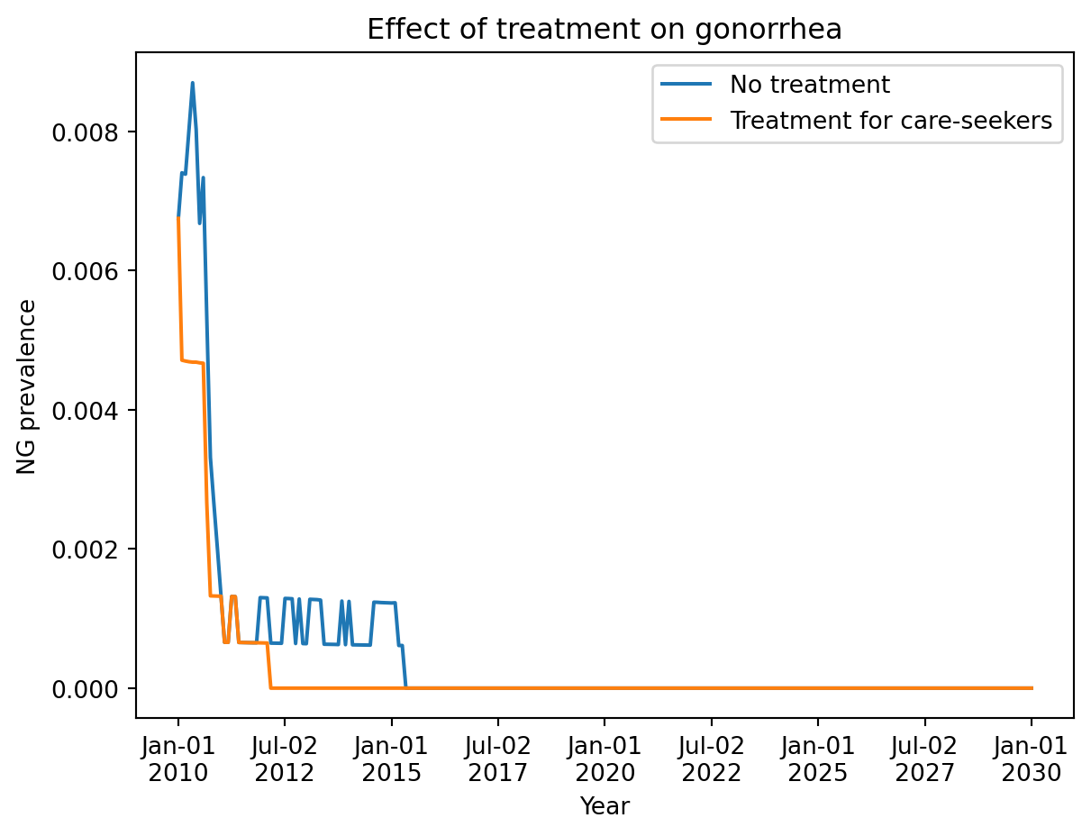
The simplest intervention pattern is a treatment with an eligibility function that determines who gets treated. Here we treat gonorrhea patients when they seek care for symptoms:
import stisim as stiimport starsim as ssimport pandas as pdimport numpy as npimport matplotlib.pyplot as plt# Baseline: no treatmentsim_base = sti.Sim(diseases='ng', n_agents=2000, start=2010, stop=2030)sim_base.run(verbose=0)# With treatment: symptomatic care-seekers get treated# ti_seeks_care is the time when an agent seeks careng = sti.Gonorrhea(init_prev=0.01)ng_tx = sti.GonorrheaTreatment( name='ng_tx', eligibility=lambda sim: sim.diseases.ng.symptomatic & (sim.diseases.ng.ti_seeks_care == sim.ti),)sim_intv = sti.Sim(diseases=ng, interventions=[ng_tx], n_agents=2000, start=2010, stop=2030)sim_intv.run(verbose=0)
Initializing sim with 2000 agents
Initializing sim with 2000 agents
fig, ax = plt.subplots()ax.plot(sim_base.timevec, sim_base.results.ng.prevalence, label='No treatment')ax.plot(sim_intv.timevec, sim_intv.results.ng.prevalence, label='Treatment for care-seekers')ax.set_xlabel('Year')ax.set_ylabel('NG prevalence')ax.set_title('Effect of treatment on gonorrhea')ax.legend()plt.show()
HIV testing and ART
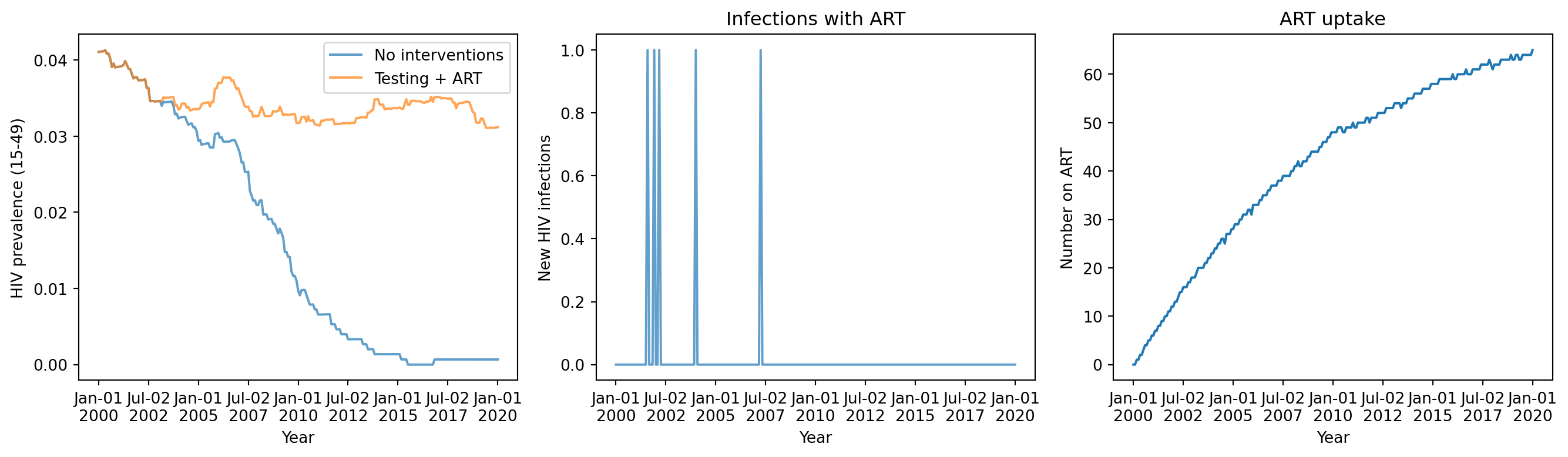
HIV interventions follow a specific pipeline: testing → diagnosis → ART initiation. Agents must be diagnosed by HIVTest before they can start ART.
Key things to know: - test_prob_data is a per-year probability, automatically scaled by timestep. With monthly dt, test_prob_data=0.1 means ~0.83% per month (~10% per year). - ART(coverage=0.8) will force-fit 80% of infected onto ART. ART() with no coverage treats everyone who is diagnosed. - art_initiation (default 90%) controls how many newly diagnosed agents are willing to start ART.
import hivsim# Simplest approach: use hivsim.demo which includes testing + ART by defaultsim_default = hivsim.demo('simple', run=False, plot=False, n_agents=3000)sim_default.run(verbose=0)# Custom: specify coverage explicitlyhiv_test = sti.HIVTest(test_prob_data=0.2, start=2000, name='hiv_test')# ART with time-varying coverage (proportion of infected)art = sti.ART(coverage={'year': [2000, 2010, 2025], 'value': [0, 0.5, 0.9]})# Without any interventions for comparisonsim_base = hivsim.demo('simple', run=False, plot=False, n_agents=3000)sim_base.pars.interventions = []sim_base.run(verbose=0)# With custom testing + ARTsim_intv = hivsim.demo('simple', run=False, plot=False, n_agents=3000)sim_intv.pars.interventions = [hiv_test, art]sim_intv.run(verbose=0)
Initializing sim with 3000 agents
Initializing sim with 3000 agents
Initializing sim with 3000 agents
fig, axes = plt.subplots(1, 3, figsize=(14, 4))axes[0].plot(sim_base.timevec, sim_base.results.hiv.prevalence_15_49, label='No interventions', alpha=0.7)axes[0].plot(sim_intv.timevec, sim_intv.results.hiv.prevalence_15_49, label='Testing + ART', alpha=0.7)axes[0].set_xlabel('Year')axes[0].set_ylabel('HIV prevalence (15-49)')axes[0].legend()axes[1].plot(sim_intv.timevec, sim_intv.results.hiv.new_infections, alpha=0.7)axes[1].set_xlabel('Year')axes[1].set_ylabel('New HIV infections')axes[1].set_title('Infections with ART')axes[2].plot(sim_intv.timevec, sim_intv.results.hiv.n_on_art)axes[2].set_xlabel('Year')axes[2].set_ylabel('Number on ART')axes[2].set_title('ART uptake')plt.tight_layout()plt.show()
Targeting interventions
Use the eligibility parameter to target interventions to specific populations. For example, FSW-targeted testing:
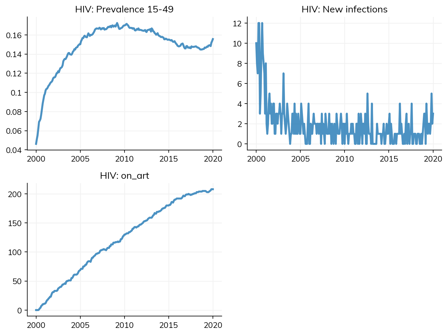
# Higher testing rate for FSWsfsw_test = sti.HIVTest( test_prob_data=0.3, start=2000, name='fsw_test', eligibility=lambda sim: sim.networks.structuredsexual.fsw &~sim.diseases.hiv.diagnosed,)# Lower testing rate for the general populationgp_test = sti.HIVTest( test_prob_data=0.05, start=2000, name='gp_test', eligibility=lambda sim: ~sim.networks.structuredsexual.fsw &~sim.diseases.hiv.diagnosed,)art2 = sti.ART(coverage=0.8)# Use StructuredSexual so `fsw` is available on the network (hivsim.demo('simple')# now uses MFNetwork by default, which has no sex-work compartment)sim = hivsim.demo('simple', run=False, plot=False, n_agents=3000, networks=[sti.StructuredSexual(), ss.MaternalNet(), ss.BreastfeedingNet()])sim.pars.interventions = [fsw_test, gp_test, art2]sim.run(verbose=0)sim.plot(key=['hiv.prevalence_15_49', 'hiv.new_infections', 'hiv.n_on_art'])
Initializing sim with 3000 agents
Figure(768x576)
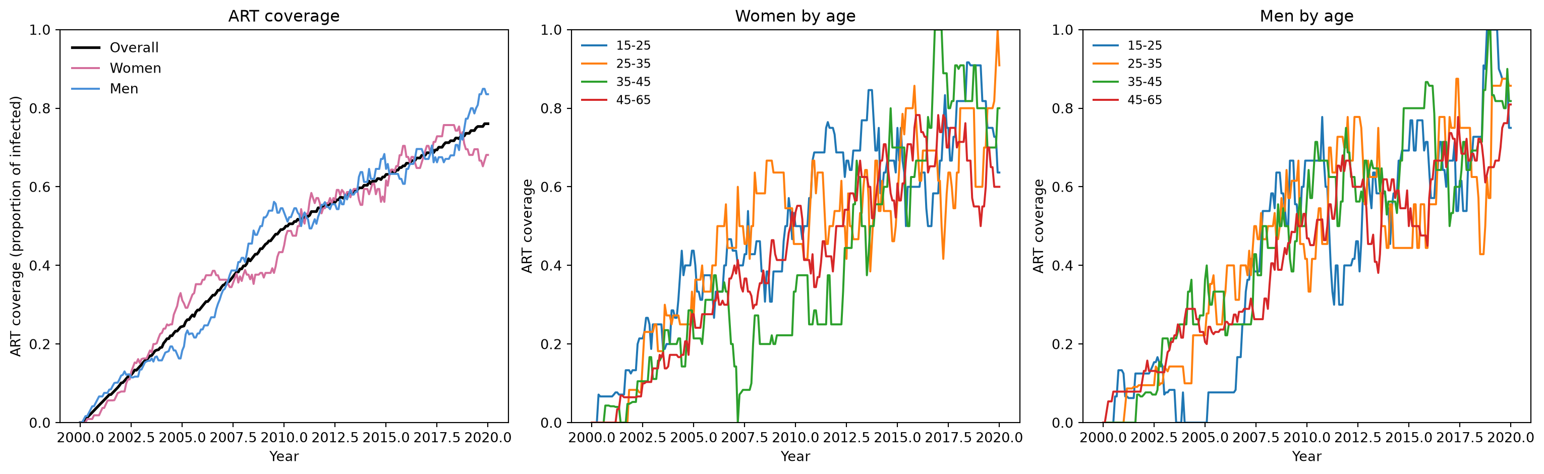
ART coverage formats and monitoring
ART accepts coverage data in several formats. You can also use the art_coverage analyzer to track coverage by age and sex, and verify that the model matches your targets.
# Different coverage formatsart_const = sti.ART(coverage=0.8) # Constant proportionart_dict = sti.ART(coverage={'year': [2000, 2010, 2025], 'value': [0, 0.5, 0.9]}) # Time-varyingart_none = sti.ART() # No target: treat all diagnosed# Run with the art_coverage analyzer to monitor coverage by age/sexsim = hivsim.demo('simple', run=False, plot=False, n_agents=5000)sim.pars.interventions = [sti.HIVTest(test_prob_data=0.3, name='hiv_test'), art_dict]sim.pars.analyzers = [sti.art_coverage(age_bins=[15, 25, 35, 45, 65])]sim.run(verbose=0)# Three ways to inspect the results:# 1. Use the built-in plot methodsim.analyzers.art_coverage.plot()# 2. Access results directlyac = sim.results.art_coverageprint(f'Final overall ART coverage: {ac.p_art[-1]:.1%}')print(f'Final coverage, women 25-35: {ac.p_art_f_25_35[-1]:.1%}')print(f'Final coverage, men 25-35: {ac.p_art_m_25_35[-1]:.1%}')# 3. Export to a DataFrame for further analysisdf = sim.results.art_coverage.to_df()print(f'\nDataFrame shape: {df.shape}')df.head()
Initializing sim with 5000 agents
Figure(1536x480)
Final overall ART coverage: 76.1%
Final coverage, women 25-35: 90.9%
Final coverage, men 25-35:   85.7%

DataFrame shape: (241, 23)
timevec
n_art
p_art
n_art_f
n_art_m
p_art_f
p_art_m
n_art_f_15_25
p_art_f_15_25
n_art_m_15_25
...
n_art_m_25_35
p_art_m_25_35
n_art_f_35_45
p_art_f_35_45
n_art_m_35_45
p_art_m_35_45
n_art_f_45_65
p_art_f_45_65
n_art_m_45_65
p_art_m_45_65
0
2000-01-01
0.0
0.000000
0.0
0.0
0.000000
0.000000
0.0
0.000000
0.0
...
0.0
0.0
0.0
0.0
0.0
0.0
0.0
0.0
0.0
0.000000
1
2000-01-31
0.0
0.000000
0.0
0.0
0.000000
0.000000
0.0
0.000000
0.0
...
0.0
0.0
0.0
0.0
0.0
0.0
0.0
0.0
0.0
0.000000
2
2000-03-02
1.0
0.004348
0.0
1.0
0.000000
0.008264
0.0
0.000000
0.0
...
0.0
0.0
0.0
0.0
0.0
0.0
0.0
0.0
1.0
0.027027
3
2000-04-02
2.0
0.008696
0.0
2.0
0.000000
0.016529
0.0
0.000000
0.0
...
0.0
0.0
0.0
0.0
0.0
0.0
0.0
0.0
2.0
0.054054
4
2000-05-02
3.0
0.013043
1.0
2.0
0.009174
0.016529
1.0
0.071429
0.0
...
0.0
0.0
0.0
0.0
0.0
0.0
0.0
0.0
2.0
0.054054
5 rows × 23 columns
Exercises
Add VMMC to the HIV sim using sti.VMMC(coverage=0.3). How does it affect new infections compared to ART alone?
Try running sti.ART() without any HIVTest — what happens? (Hint: check for a warning.)
Compare sti.ART(coverage=0.5) vs sti.ART(coverage=0.9) — how does the number on ART differ? Use sti.art_coverage() to plot the results.
Create a sim with both gonorrhea and chlamydia, and use a single STITreatment(diseases=['ng', 'ct']) to treat both. Compare prevalence with and without treatment.