Results and plotting

This tutorial covers how to inspect, export, and plot results from an STIsim simulation.

Setup

Let’s run a simple gonorrhea simulation to work with:

import stisim as sti
import matplotlib.pyplot as plt

sim = sti.Sim(diseases='ng', n_agents=2000, start=2010, stop=2030)
sim.run(verbose=0)

Initializing sim with 2000 agents

Sim(n=2000; 2010—2030; networks=structuredsexual, maternalnet; diseases=ng)

Browsing available results

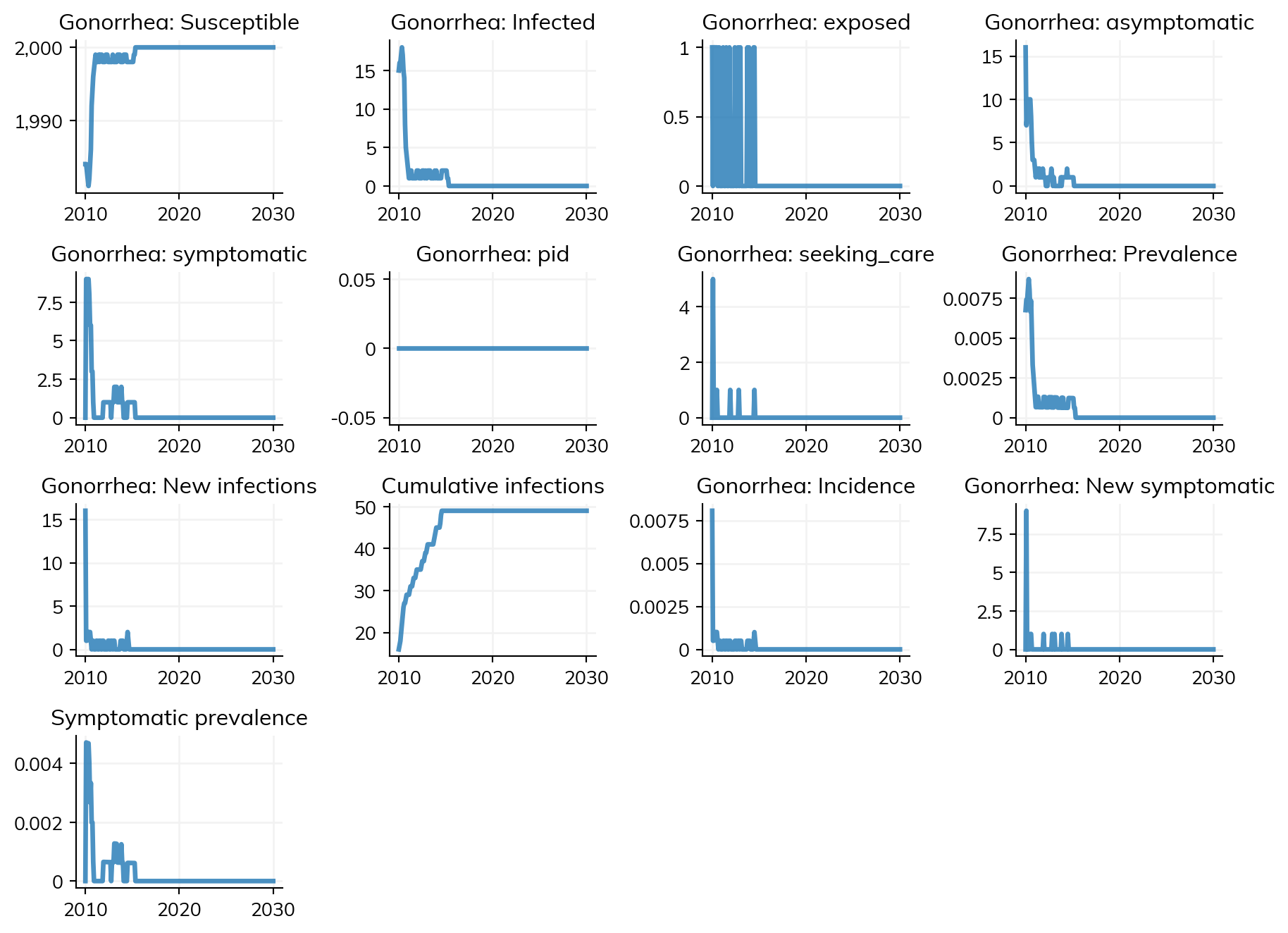
After running a sim, all results are stored in sim.results. Each disease has its own results object. You can list all available keys with sim.results.ng.keys(), or access individual results directly. STIsim stores results at multiple levels of detail: overall, by sex, and by age group.

# Access individual results
prev = sim.results.ng.prevalence
print(f'{prev.label}: min={prev.values.min():.3f}, mean={prev.values.mean():.3f}, max={prev.values.max():.3f}')

new_inf = sim.results.ng.new_infections
print(f'{new_inf.label}: min={new_inf.values.min():.0f}, mean={new_inf.values.mean():.1f}, max={new_inf.values.max():.0f}')

# There are many more -- including by sex and age group
print(f'\nTotal result keys: {len(sim.results.ng.keys())}')

Prevalence: min=0.000, mean=0.001, max=0.009
New infections: min=0, mean=0.2, max=16

Total result keys: 204

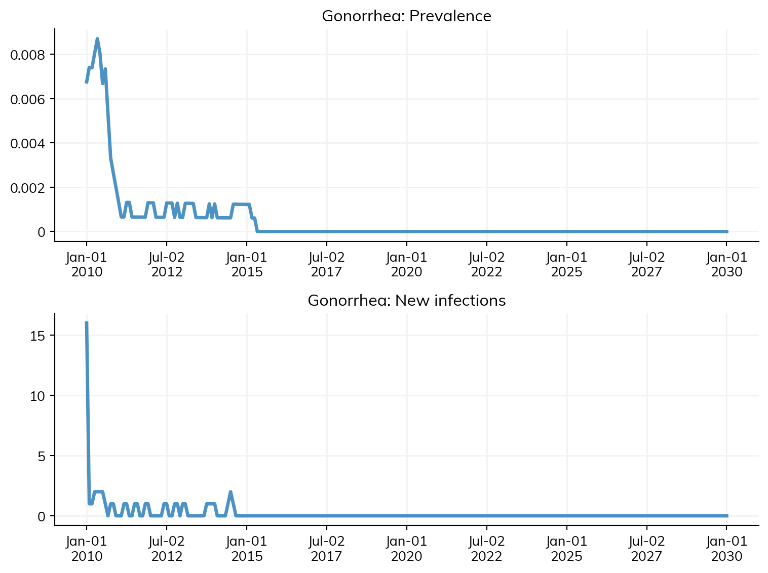
Each result is an ss.Result object. The raw data is in .values (a NumPy array) and the time axis is in .timevec:

print(f'Values (first 5): {prev.values[:5]}')
print(f'Timevec:          {prev.timevec[0]} to {prev.timevec[-1]} ({len(prev.values)} timesteps)')

Values (first 5): [0.00675219 0.00740741 0.00738751 0.0080429  0.00870147]
Timevec:          2010.01.01 to 2030.01.01 (241 timesteps)

Automatic plotting

The simplest way to visualize results is sim.plot(). By default, it shows only the high-level results (not every age/sex subgroup):

sim.plot()

Figure(896x672)

Plotting specific results

To plot specific results, pass the key argument. You can use a single key or a list:

# Plot just prevalence and new infections
sim.plot(key=['ng.prevalence', 'ng.new_infections'])

Figure(768x576)

You can also plot results that are hidden from the default view. For example, sex-stratified prevalence:

sim.plot(key=['ng.prevalence_f', 'ng.prevalence_m'])

Figure(768x576)

Exporting results

As a DataFrame

Export all results to a Pandas DataFrame with sim.to_df():

df = sim.to_df()
print(f'Shape: {df.shape}')
df.head()

Shape: (241, 211)

	timevec	structuredsexual_n_edges	ng_n_susceptible	ng_n_infected	ng_n_exposed	ng_n_asymptomatic	ng_n_symptomatic	ng_n_seeking_care	...	ng_new_symptomatic_m_50_65	ng_symp_prevalence_m_50_65	n_alive
0	2010-01-01	228.0	1984.0	15.0	1.0	16.0	0.0	0.0	...	0.0	0.000000	2000.0
1	2010-01-31	267.0	1984.0	16.0	0.0	7.0	9.0	5.0	...	1.0	0.005988	2000.0
2	2010-03-03	365.0	1983.0	16.0	1.0	8.0	9.0	0.0	...	0.0	0.005952	2000.0
3	2010-04-02	398.0	1982.0	17.0	1.0	9.0	9.0	1.0	...	0.0	0.005917	2000.0
4	2010-05-03	398.0	1981.0	18.0	1.0	10.0	9.0	0.0	...	0.0	0.005780	2000.0

5 rows × 211 columns

You can also export a single result:

prev_df = sim.results.ng.prevalence.to_df()
prev_df.head()

	timevec	value
0	2010-01-01	0.006752
1	2010-01-31	0.007407
2	2010-03-03	0.007388
3	2010-04-02	0.008043
4	2010-05-03	0.008701

Resampling to annual results

STIsim runs with monthly timesteps by default, but you’ll often want annual results for reporting or comparison with data. Use the resample() method on any result:

# Monthly new infections (raw)
monthly = sim.results.ng.new_infections
print(f'Monthly: {len(monthly.values)} timesteps')

# Resample to annual (sums monthly counts)
annual = monthly.resample('year')
print(f'Annual:  {len(annual)} years')
print(annual)

Monthly: 241 timesteps
Annual:  21 years
Result(Gonorrhea.new_infections: min=0, mean=2.33333, max=29)

The resample() method automatically chooses the right aggregation: sum for counts (like new_infections) and mean for rates/proportions (like prevalence). You can also resample to a DataFrame:

annual_df = sim.results.ng.new_infections.resample('year')
print(f'Annual result: {len(annual_df.values)} years')
print(annual_df)

Annual result: 21 years
Result(Gonorrhea.new_infections: min=0, mean=2.33333, max=29)

You can also resample the entire sim’s results at once via to_df():

annual_all = sim.to_df(resample='year', use_years=True)
annual_all.head()

	timevec	structuredsexual_n_edges	ng_n_susceptible	ng_n_infected	ng_n_exposed	ng_n_asymptomatic	ng_n_symptomatic	ng_n_seeking_care	...	ng_new_symptomatic_m_50_65	ng_symp_prevalence_m_50_65	n_alive
0	2010	393.833333	1987.083333	12.333333	0.583333	7.666667	5.250000	0.583333	...	1.0	0.002446	2000.0
1	2011	472.166667	1998.416667	1.333333	0.250000	1.500000	0.083333	0.083333	...	0.0	0.000000	2000.0
2	2012	488.666667	1998.333333	1.500000	0.166667	0.750000	0.916667	0.083333	...	0.0	0.000000	2000.0
3	2013	499.583333	1998.333333	1.416667	0.250000	0.250000	1.416667	0.000000	...	0.0	0.000000	2000.0
4	2014	513.166667	1998.333333	1.500000	0.166667	1.083333	0.583333	0.083333	...	0.0	0.000000	2000.0

5 rows × 211 columns

Custom plots with Matplotlib

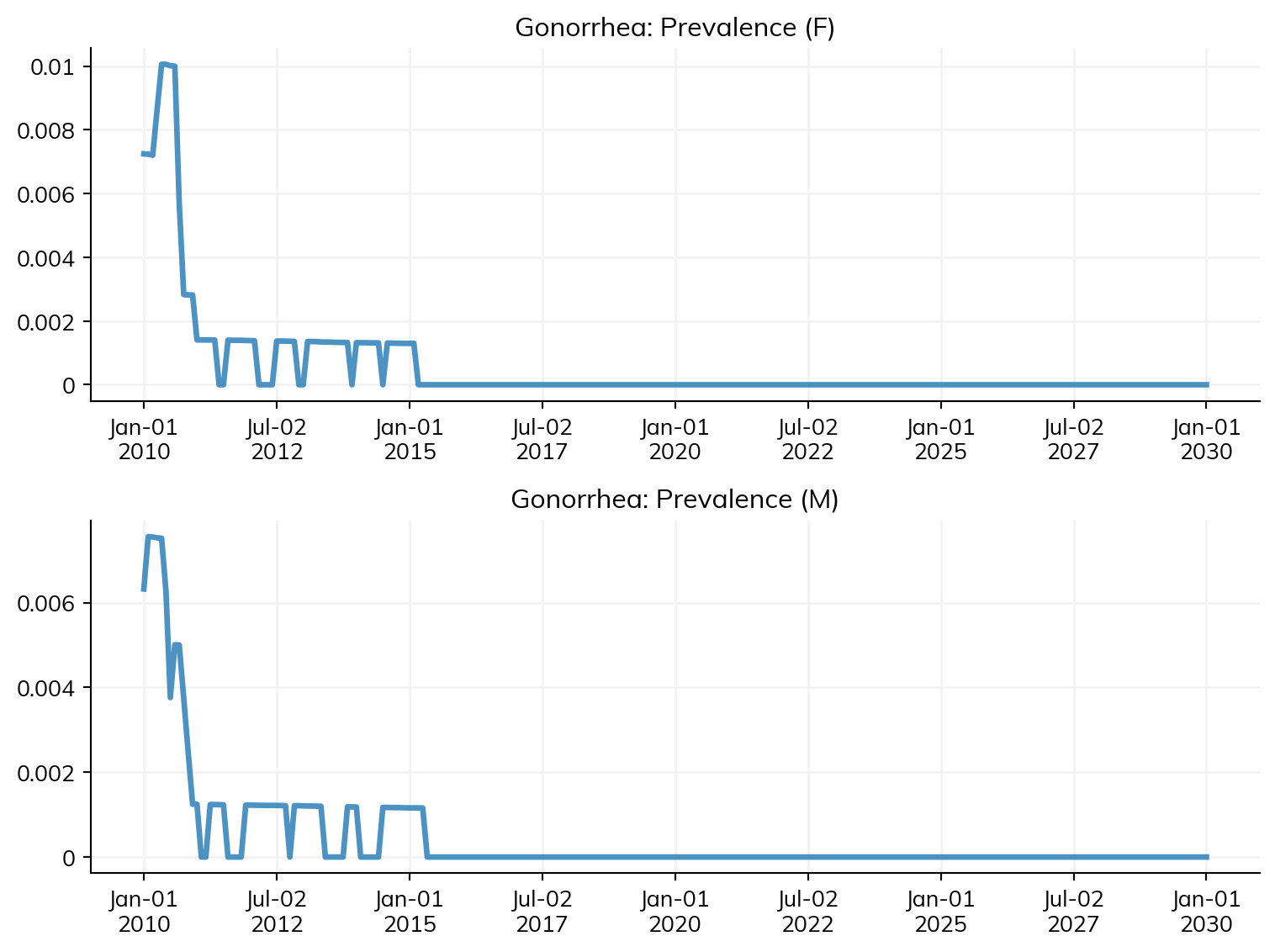
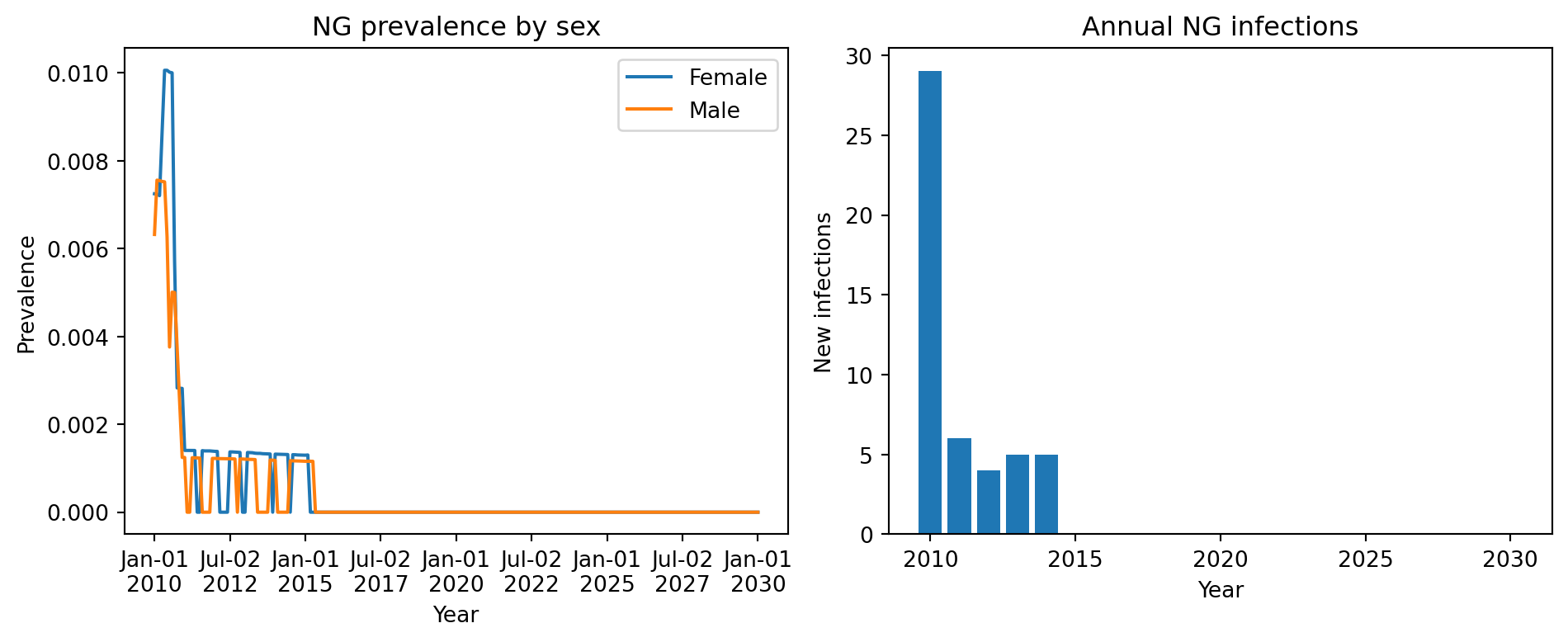
For publication-quality figures or custom layouts, use the result values directly with Matplotlib:

fig, axes = plt.subplots(1, 2, figsize=(10, 4))

# Left: prevalence by sex
axes[0].plot(sim.timevec, sim.results.ng.prevalence_f, label='Female')
axes[0].plot(sim.timevec, sim.results.ng.prevalence_m, label='Male')
axes[0].set_xlabel('Year')
axes[0].set_ylabel('Prevalence')
axes[0].set_title('NG prevalence by sex')
axes[0].legend()

# Right: annual new infections (resampled)
annual_inf = sim.results.ng.new_infections.resample('year', use_years=True)
axes[1].bar(annual_inf.timevec, annual_inf.values)
axes[1].set_xlabel('Year')
axes[1].set_ylabel('New infections')
axes[1].set_title('Annual NG infections')

plt.tight_layout()
fig

## Custom results

STIsim’s built-in results cover the most common quantities (prevalence, incidence, counts by sex and age group). But you’ll often need something specific to your analysis – coinfection prevalence in a subgroup, treatment coverage by pathway, network contact rates, etc.

Any module can define custom results: analyzers, interventions, networks, connectors, and diseases all use the same define_results pattern. The result then automatically appears in sim.results, sim.to_df(), and sim.plot() – and can be used as a calibration target.

Here’s a minimal example using an analyzer that tracks gonorrhea prevalence among people aged 15-24:

import starsim as ss

class YouthPrev(ss.Analyzer):
    """Track gonorrhea prevalence among 15-24 year olds."""

    def init_pre(self, sim):
        super().init_pre(sim)
        # define_results registers a result with the sim's results system.
        # After sim.run(), it appears in sim.results.youthprev.ng_prev_15_24
        # and in sim.to_df() as 'youthprev.ng_prev_15_24'.
        self.define_results(
            ss.Result('ng_prev_15_24', dtype=float, scale=False, label='NG prev (15-24)'),
        )

    def step(self):
        ppl = self.sim.people
        youth = (ppl.age >= 15) & (ppl.age < 25)       # Boolean mask for 15-24 year olds
        n_youth = youth.count()                          # How many are in this group
        if n_youth > 0:
            infected = self.sim.diseases.ng.infected     # Boolean: who is infected
            prev = (infected & youth).count() / n_youth  # Prevalence = infected / total
            self.results['ng_prev_15_24'][self.ti] = prev

How it works:

init_pre is called during sim.init(). Call self.define_results(...) to register your results. Each ss.Result gets a pre-allocated array matching the simulation’s number of timesteps. The result is stored under sim.results.<module_name>.<result_name> – in this case, sim.results.youthprev.ng_prev_15_24.
step is called every timestep. Access the sim via self.sim, compute your quantity, and store it in self.results[name][self.ti] where self.ti is the current timestep index.
After sim.run(), the result is available everywhere: sim.results, sim.to_df(), sim.plot(), and as a calibration target (see Calibration tutorial).

This same pattern works in any module – interventions, connectors, networks, etc. Anywhere you can write define_results in init_pre and self.results[name][self.ti] = value in step, you get a tracked result.

`ss.Result` options

The most commonly used arguments to ss.Result:

Argument	Default	Description
`name`	(required)	Key used to access the result, e.g. `'ng_prev_15_24'`
`dtype`	`float`	Data type (`float` for rates, `int` for counts)
`scale`	`True`	Whether to scale the result when changing `n_agents`. Set `True` for counts (e.g., new infections), `False` for rates/proportions (e.g., prevalence)
`auto_plot`	`True`	Whether to include in `sim.plot()` by default. Set `False` for results you only need in `to_df()`
`label`	`None`	Human-readable label for plot axes

Let’s try it:

# Run a sim with our custom analyzer
sim = sti.Sim(diseases='ng', n_agents=2000, start=2010, stop=2030, analyzers=[YouthPrev()])
sim.run(verbose=0)

# The result is now accessible like any built-in result
print(sim.results.youthprev.ng_prev_15_24)

# And it shows up in to_df()
df = sim.to_df(resample='year', use_years=True, sep='.')
print(df[['timevec', 'youthprev.ng_prev_15_24']].head())

Initializing sim with 2000 agents
Result(YouthPrev.ng_prev_15_24: min=0, mean=0, max=0)
   timevec  youthprev.ng_prev_15_24
0     2010                      0.0
1     2011                      0.0
2     2012                      0.0
3     2013                      0.0
4     2014                      0.0

Summary

Task	Method
List all result keys	`sim.results.ng.keys()`
Access a result’s values	`sim.results.ng.prevalence.values`
Auto-plot high-level results	`sim.plot()`
Plot specific results	`sim.plot(key=['ng.prevalence', 'ng.new_infections'])`
Plot hidden results	`sim.plot(key='ng.prevalence_f')`
Export all to DataFrame	`sim.to_df()`
Export one result	`sim.results.ng.prevalence.to_df()`
Resample to annual	`result.resample('year')`
Annual DataFrame	`sim.to_df(resample='year', use_years=True)`
Add custom result	Write an `ss.Analyzer` with `define_results`

Exercises

Run a sim with both 'ng' and 'ct'. Use sim.plot(key=...) to compare the prevalence of the two diseases on the same figure.
Export the annual new infections for gonorrhea to a DataFrame and save it to a CSV file.
Make a Matplotlib figure that plots monthly symptomatic prevalence (ng.symp_prevalence) alongside total prevalence (ng.prevalence). What fraction of infections are symptomatic?
Write an analyzer that tracks the number of symptomatic gonorrhea cases in males aged 25-49. Run the sim with it and verify the result appears in sim.to_df().